Tag: projects

I recently took the CICS Make course available at the University of Massachusetts Amherst with my colleague Hannah Dacayanan. At the end of the course we were required to build a final project that involved interacting with the physical world using computers.

We decided to build a robot cat. More specifically, a small motorized car that would follow a laser emitted from a laser pointer around a flat surface. This was inspired by popular viral online videos of real cats trying to pounce on red dots from laser pointers.

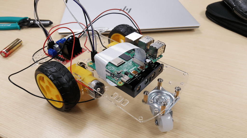
Hardware

The first thing that needed to be done was to get all the hardware and put it together. The main four components used were a car kit provided to us by the class, a Raspberry Pi 4, the Raspberry Pi camera, and the L298N motor driver.

Hannah assembled the car kit over our Thanksgiving break and I attached the L298N driver and Raspberry Pi via the Pi’s onboard GPIO pins.

We used six GPIO pins from the Raspberry Pi to control the motors, the first three (11, 13, 15) for the left, and the last three (19, 21, 23) for the right.

At this point the hardware is completely done.

Software

For the cat to follow the laser, we needed some software on the Raspberry Pi to take a frame from the camera and tell us where in that frame the laser is, if at all.

There are two possible approaches to take: deep learning or hand-crafted algorithm. We opted to try the deep learning approach first.

Lasernet

To build a neural network that can both recognize and localize lasers in an image we decided to use TensorFlow. We didn’t want to have to label tons of training data and generating synthetic data yielded poor results, so instead we went to with a semi-supervised network. Lasernet takes as input a frame of video and outputs the likelihood of a laser existing in the image. In the network there is an attention mechanism used which is where we will get our localization properties form.

First let’s import everything

from tensorflow.keras.models import Model
from tensorflow.keras.layers import (
	Input,
	Conv2D,
	Activation,
	Reshape,
	Flatten,
	Lambda,
	Dense,
)
from tensorflow.keras.callbacks import ModelCheckpoint
import tensorflow.keras.backend as K

Then we can define some global settings that are useful for us to use in the network

# Settings
IMG_SHAPE = (128, 128, 3)
FILTERS = 16
DEPTH = 0
KERNEL = 8
BATCH_SIZE = 32

Now, we get to actually building the network. The first layer is the input for our image at the resolution specified in the settings (currently 128×128), then the second is a 2d convolutional layer using the number of filters and kernel specified in the settings.

‘same’ padding is used to keep the output of the convolutional layer the same shape as its input. This is important for when the network outputs a probability distribution for each pixel in the attention mechanism.

encoder_input = Input(shape=IMG_SHAPE)
encoder = Conv2D(FILTERS, KERNEL, activation='relu', padding='same', name='encoder_conv_0')(encoder_input)

You could optionally add more convolutional layers to the network with the following code

for i in range(DEPTH):
	encoder = Conv2D(FILTERS, KERNEL, activation='relu', padding='same', name=f'encoder_conv_{i + 1}')(encoder)

Although, in our production model settings the ‘DEPTH’ is set to zero, which just uses the first convolutional layer.

Next, we write the attention mechanism. Attention shows us where the neural network “looks” to determine whether there exists a laser in the image or not. In theory, the pixel with the highest attention weight should be where the laser is.

attention_conv = Conv2D(1, KERNEL, activation='relu', padding='same', name='attention_conv')(encoder)
attention_flatten = Flatten(name='attention_flatten')(attention_conv)
attention_softmax = Activation('softmax', name='attention_softmax')(attention_flatten)
attention_reshape = Reshape((IMG_SHAPE[0], IMG_SHAPE[1], 1), name='attention_reshape')(attention_softmax)
attention_output = Lambda(lambda x : x[0] * x[1], name='attention_output')([encoder_input, attention_reshape])

There is a lot going on in that code, but basically here’s what each layer does:

• Attention Conv: takes an image or output of another convolutional layer and transforms it in some way that is learned by the neural network. In this case it will output a 128×128 matrix.
• Attention Flatten: flattens the 128×128 matrix into a 16,384 item vector.
• Attention Softmax: applies softmax activation to the vector and outputs another 16,384 item long vector with values between 0 and 1 that sum to 1. The i’th item of this vector is the weight of the i’th pixel in the input.
• Attention Reshape: reshapes the softmax vector be the input resolution.
• Attention Output: multiply the pixel weights by the pixels element wise. Pixels with higher weights will be preserved more while those with lower weights will not.

Now, we just need to get all of the outputs setup.

classifier1_flatten = Flatten(name='classifier1_flatten')(attention_reshape)
classifier2_flatten = Flatten(name='classifier2_flatten')(attention_output)
classifier1 = Lambda(lambda x : K.max(x, axis=-1), name='classifier1')(classifier1_flatten)
classifier2 = Dense(1, activation='sigmoid', name='classifier2')(classifier2_flatten)

Again here is a summary of each layer:

• Classifier 1 Flatten: converts the attention weight matrix to a vector again (this is equivalent to the Attention Softmax layer)
• Classifier 2 Flatten: converts the output of the attention mechanism to a vector
• Classifier 1: Outputs the maximum probability of the attentions weights
• Classifier 2: Uses a general feed-forward dense layer to learn how to “see” a laser.

Both classifiers will be trained to predict whether there is a laser in the input image and output either a 1 or 0. Classifier 1 forces the attention mechanism to produce a weight greater than 0.5 when there does exist a laser and product all weights less than 0.5 when there does not exist a laser. Classifier 2 is used for laser detection in production.

Finally, there is one last part of the network. We have it try to reconstruct the original image from just the attention weights. The idea here is that the easiest thing for the network to reconstruct should be the laser (since that’s the only thing in common between all images) which should encourage the attention mechanism to highlight that in the weights.

decoder = Conv2D(FILTERS, KERNEL, activation='relu', padding='same', name='decoder')(attention_reshape)
decoder = Conv2D(IMG_SHAPE[2], KERNEL, activation='relu', padding='same', name='decoder_output')(decoder)

The last thing needed is to compile the model. We use binary cross entropy for the two classifiers and mean squared error for the reconstruction loss. The optimizer is Adam.

model = Model(encoder_input, [classifier1, classifier2, decoder])
model.compile(
	loss=['binary_crossentropy', 'binary_crossentropy', 'mse'],
	loss_weights=[1000, 1000, 1],
	optimizer='adam',
	metrics=['accuracy']
)

Generating Training Data

I won’t go over the code for loading and reading the training data, but you can find the complete training script here. That said, there are a few interesting things we did in preprocessing.

Recall that, in production Lasernet is fed a continuous stream of frames from the Raspberry Pi camera. So what we do is take the average of the previous 10 frames and diff that with the current frame. Then send the diff the Lasernet instead of the raw frame.

This produces images where anything that is not really moving tends to be blacked out.

Train it

It’s training time! I trained Lasernet on my Nvidia GeForce GTX 1060 6GB for a day or so and here is the result.

The white dot is the network’s prediction for each frame, and the red circle is the moving average of predictions.

Catcarlib

Now, that the neural network is done, we needed some library for actually driving the car using the GPIO pins on the Raspberry Pi. For this purpose, we created catcarlib.

First we use the Raspberry Pi GPIO Python library to help us in controlling the pins on the board. Let’s import that.

import RPi.GPIO as GPIO 

Next, we need to initialize GPIO with the correct pins that are connected to the car. In our case those were:

• Left Motor Power: 11
• Left Motor Forward: 13
• Left Motor Backward: 15
• Right Motor Power: 23
• Right Motor Forward: 21
• Right Motor Backward: 19

channels = [
	{'label': 'LEFT_MOTOR_POWER', 'pin': 11},
	{'label': 'LEFT_MOTOR_FORWARD', 'pin': 13},
	{'label': 'LEFT_MOTOR_BACKWARD', 'pin': 15},
	{'label': 'RIGHT_MOTOR_POWER', 'pin': 23},
	{'label': 'RIGHT_MOTOR_FORWARD', 'pin': 21},
	{'label': 'RIGHT_MOTOR_BACKWARD', 'pin': 19},
]

GPIO.setmode(GPIO.BOARD)
GPIO.setup([i['pin'] for i in channels], GPIO.OUT, initial=GPIO.LOW)
state = [False for i in channels]

To review, we set the GPIO mode to use the pin numbers on the board. Then we setup each pin in channels and initialize it to 0. The state list is used to keep track of what the current state of each pin is.

Now it would be good to write some helper functions for things like resetting all the pins, get the index for each action in the state, and enabling pins.

def reset(state):
	for i in range(len(state)):
		state[i] = False

def getIndexFromLabel(label):
	for i, channel in enumerate(channels):
		if channel['label'] == label:
			return i

	return None

def commit(state):
	GPIO.output([i['pin'] for i in channels], state)

def enableByLabel(state, labels):
	for label in labels:
		state[getIndexFromLabel(label)] = True

• reset: resets the states to all zero
• getIndexFromLabel: gets the index of a particular action in the state list
• commit: sends the current state to the pins
• enableByLabel: enables a list of actions

At last, we can write the functions to actually move the car. Below is the function for moving the car forward. First it resets the state to a blank slate of all zeros. Then it enables the power for both motors and the forward pins. Finally, it commits the changes to the GPIO pins.

def forward():
	reset()
	enableByLabel([
		'LEFT_MOTOR_POWER',
		'LEFT_MOTOR_FORWARD',
		'RIGHT_MOTOR_POWER',
		'RIGHT_MOTOR_FORWARD',
	])
	commit()

The functions for left, right, and backwards can be written in much the same way. For left we want to left wheel to go forward, and the right wheel to go backward. Going right is the opposite of left, and going backward is the opposite of going forward.

Again you can see the full catcarlib.py on GitHub.

Putting everything together

So, now we have all the hardware ready, Lasernet trained, and catcarlib to control the car. Let’s see how it does.

To be honest with you, I was a little disappointed with the performance at this point. I was just hoping for more.

I tried a number of different things to improve the performance. Sanity checks to reduce false positives like checking the color of the pixel where the network predicted the laser to be, or the euclidean distance between the prediction and the images brightest pixel.

Ultimately nothing worked well enough to bring the performance to where I wanted it to be.

Catseelib

Since the neural network approach didn’t seem to be working out I decided try to come up with some handcrafted algorithm that can do it. I’ll call it catseelib.

The approach of taking the diff between the current frame and the average of the last 10 was pretty useful, so let’s start there. Then we can just take the pixel with the highest magnitude in the diff. That should be the laser if there is minimal background noise.

To make sure that the only thing in the diff was the laser, I pointed the camera straight down under the head of the cat. Let’s see how well that works.

Good enough, let’s give Hannah a try.